Rでヒストグラム(hist)

Rのグラフィックスを使ってヒストグラムを作成します。ヒストグラムは連続量を構造をみるのに有用です。仕組みとしては連続量を決まった間隔毎にわけ、その間隔ごとの件数をみることができます。細かな設定もみていきましょう。

# データサンプルとして正規分布で乱数発生
 x <- rnorm(1000,mean = 0,sd = 1)
# ヒストグラム
 hist(x = x)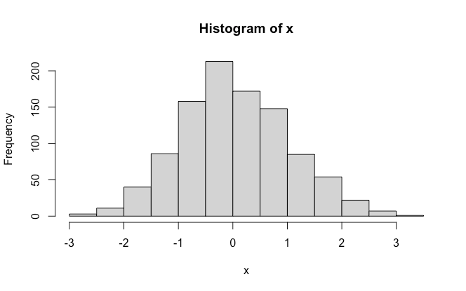

階級幅の変更

breaksにひとつだけ数値をいれるとその階級幅でヒストグラムを作成してくれます。

hist(x = x,breaks = c(-9-1,3,2,1,10))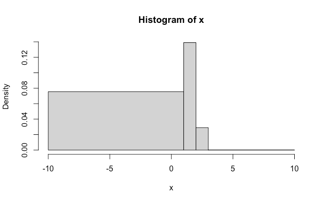

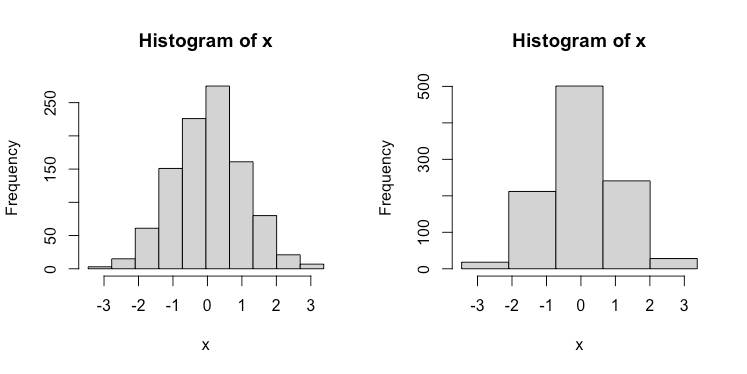
階級幅（10分割）

par(mfrow = c(1,2))
 hist(x = x,breaks = seq(min(x),max(x),length.out = 11)) # 10分割
 hist(x = x,breaks = seq(min(x),max(x),length.out = 6)) # 5分割

タイトル設定、色変更

par(mfrow = c(1,2))
 hist(x = x,main = "title test",xlab = "text x",ylab = "text y")
 hist(x = x,col = "blue")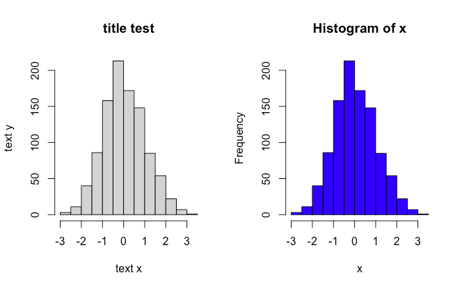

確率表示

hist(x = x,main = "title test",freq = T)
 hist(x = x,main = "title test",freq = F)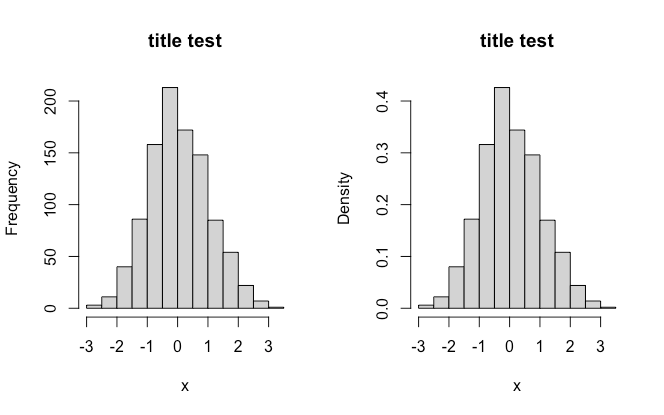

横幅、縦幅の調整

par(mfrow = c(2,2))
 hist(x = x,main = "title test")
 hist(x = x,main = "title test",xlim = c(-2,6))
 hist(x = x,main = "title test",ylim = c(0,500))
 hist(x = x,main = "title test",xlim = c(-2,6),ylim = c(0,500),freq = F)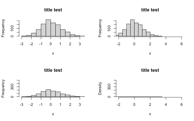

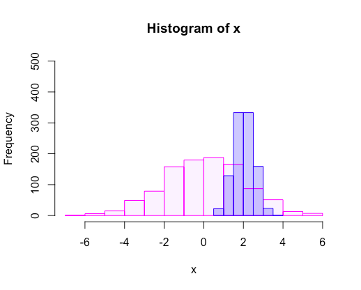
重ね合わせ

# 変数追加
 x <- rnorm(1000,mean = 0,sd = 2)
 y <- rnorm(1000,mean = 2,sd = 0.5)
# 重ね合わせ
 par(mfrow = c(1,1))
 hist(x, col = "#aa00ff10", border = "#ff00ff",ylim = c(0,500),freq = T)
 hist(y, col = "#0000ff40", border = "#0000ff",ylim = c(0,500), add = TRUE,freq = T)